Contents

Profile Estimation Experiments - General Forced Linear Systems

This page details the use of the 'genlin' functions with the profiling code to estimate parameters in a general class of forced linear differential equations. The file largely follows the structure of FhnEx.html and the reader is referred there and to the Profile Users Manual for commentary not specifically associated with forced linear systems.

These functions are set up to deal with equations of the form

where u is a known vector of forcing functions and the parameters occur as entries in A and B.

Note that the dimensions of x and u are detected automatically.

% The function to input into the ODE solver is

odefn       = @genlinfunode;    % Function for ODE solver (exact)

RHS Functions

We define the genlin library specifically here:

fn.fn       = @genlinfun;       % RHS function
fn.dfdx     = @genlindfdx;      % Derivative wrt inputs (Jacobian)
fn.dfdp     = @genlindfdp;      % Derviative wrt parameters

fn.d2fdx2   = @genlind2fdx2;    % Hessian wrt inputs
fn.d2fdxdp  = @genlind2fdxdp;   % Hessian wrt inputs and parameters
fn.d2fdp2   = @genlind2fdp2;    % Hessian wrt parameters.

fn.d3fdx3   = @genlind3fdx3;    % Third derivative wrt inputs.
fn.d3fdx2dp = @genlind3fdx2dp;  % Third derivative wrt intputs, inputs and pars.
fn.d3fdxdp2 = @genlind3fdxdp2;  % Third derivative wrt inputs, pars and pars.
                                % dimensions = time, component, input,
                                % parameters

Various parameters

The main input into genlin that needs to be tailored is a component labelled more. This controls which elements of which matrices will be estimated. If left empty, it assumes that there is no forcing component u and the all the elements of A must be estimated.

Where it is not the case that all elements of A must be estimated, more is a struct with the following entries:

% In the following, we have a 2-by-2 system in which A(2,1) is specified as
% zero and is not estimated:

more = [];
more.mat = zeros(2,2);
more.sub = [1 1; 1 2; 2 2];         % Specify that A(2,1) is zero and
                                    % not being estimated.

% The rest of the parameters can be specified as normal.

y0 = [-1,1];                    % Initial conditions

pars = [-1; 2; -1; 1; -1];      % Parameters (final two used for forcing
disp(['Parameter values: ',num2str(pars')]);       % functions).

sigma = 0.1;                    % Noise Level

jitter = 0.2;                                % Perturbation for starting
startpars = pars + jitter*randn(length(pars),1); % of parameter estimates
disp('Initial parameter values: ')
disp(num2str(startpars'));       % functions).

Parameter values: -1  2 -1  1 -1
Initial parameter values: 
-1.0692      2.1063    -0.70081      1.2718     -1.0128

Forcing components

If the system is forced, then a number of other components of more must be specified:

If more.force is not specified, then the system is assumed to be autonomous.

% In the following, the first component is forced by 'sinin'; a sin
% function, and the second component by a constant.

more.force = {@sinin,fd(3,create_constant_basis(2))};
more.force_mat = zeros(2,2);
more.force_sub = [1 1; 2 2];

% The rest of the estimation can now proceed as normal.

Observation times

tspan = 0:0.005:2;    % Observation times

obs_pts{1} = 1:length(tspan);      % Which components are observed at
obs_pts{2} = 1:length(tspan);      % which observation times.

tfine = 0:0.005:2;    % Times to plot solutions

Calculate trajectories

odeopts = odeset('RelTol',1e-13);
[full_time,full_path] = ode45(odefn,tspan,y0,odeopts,pars,more);
[plot_time,plot_path] = ode45(odefn,tfine,y0,odeopts,pars,more);

Set up observations

Tcell = cell(1,size(full_path,2));
path = Tcell;

for i = 1:length(obs_pts)
    Tcell{i} = full_time(obs_pts{i});
    path{i} = full_path(obs_pts{i},i);
end

% add noise

Ycell = path;
for i = 1:length(path)
    Ycell{i} = path{i} + sigma*randn(size(path{i}));
end

% *Set up weights*

wts = [];
if isempty(wts)                             % estimate wts if not given
    for i = 1:length(Ycell)
        wts(i) = 1./sqrt(var(Ycell{i}));
    end
end

Fitting parameters

lambda  = 1e4;   % Smoothing for model-based penalty
lambda  = lambda*wts;

lambda0 = 1e0;   % Smoothing for 1st-derivative penalty

nknots = 401;    % Number of knots to use.
nquad  = 5;      % No. between-knots quadrature points.
norder = 3;      % Order of B-spline approximation

Profiling optimisation control

maxit1 = 1000;      % Maximum iterations interior of profiling
maxit0 = 1000;      % Maximum iterations for outer optimization

lsopts_out = optimset('DerivativeCheck','on','Jacobian','on',...
    'Display','iter','MaxIter',maxit0,'TolFun',1e-8,'TolX',1e-10);

% Other observed optimiation control
lsopts_other = optimset('DerivativeCheck','off','Jacobian','on',...
    'Display','iter','MaxIter',maxit0,'TolFun',1e-14,'TolX',1e-14,...
    'JacobMult',@SparseJMfun);

% Optimiation control within profiling
lsopts_in = optimset('DerivativeCheck','off','Jacobian','on',...
    'Display','off','MaxIter',maxit1,'TolFun',1e-14,'TolX',1e-14,...
    'JacobMult',@SparseJMfun);

Setting up functional data objects

% set up knots

range = [min(full_time),max(full_time)];  % Range of observations

knots_cell = cell(size(path));     % Knots for each basis
knots_cell(:) = {linspace(range(1),range(2),nknots)};

% set up bases

basis_cell = cell(1,length(path)); % Create cell arrays.
Lfd_cell = cell(1,length(path));

nbasis = zeros(length(path),1);

bigknots = knots_cell{1};          % bigknots used for quadrature points
nbasis(1) = length(knots_cell{1}) + norder - 2;

for i = 2:length(path)
    bigknots = [bigknots knots_cell{i}];
    nbasis(i) = length(knots_cell{i}) + norder -2;
end

quadvals = MakeQuadPoints(bigknots,nquad);   % Create simpson's rule
                                             % quadrature points and values
for i = 1:length(path)
    basis_cell{i} = MakeBasis(range,nbasis(i),norder,...  % create bases
        knots_cell{i},quadvals,1);                        % with quadrature
    Lfd_cell{i} = fdPar(basis_cell{i},1,lambda0);         % pts  attatched
end

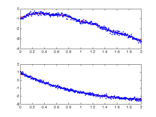
Smooth the data

DEfd = smoothfd_cell(Ycell,Tcell,Lfd_cell);
coefs = getcellcoefs(DEfd);

devals = eval_fdcell(tfine,DEfd,0);
for i = 1:length(path)
    subplot(length(path),1,i);
    plot(tfine,devals{i},'r','LineWidth',2);
    hold on;
    plot(Tcell{i},Ycell{i},'b.');
    hold off;
end

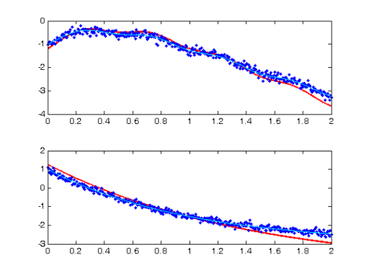
Re-smoothing with model-based penalty

% Call the Gauss-Newton solver

[newcoefs,tDEfd] = genlin_smooth(path,Tcell,[],basis_cell,lambda,startpars,[],more);

% Plot results along with exact solution

devals = eval_fdcell(tfine,tDEfd,0);
for i = 1:length(path)
    subplot(length(path),1,i);
    plot(tfine,devals{i},'r','LineWidth',2);
    hold on;
    plot(Tcell{i},Ycell{i},'b.');
    plot(plot_time,plot_path(:,i),'c');
    hold off
end

Perform the Profiled Estimation

[newpars,newDEfd_cell] = Profile_GausNewt(startpars,lsopts_out,tDEfd,fn,...
    lambda,Ycell,Tcell,wts,[],lsopts_in,more);

disp('New parameter values:')
disp(newpars');

 Iteration       steps    Residual   Improvement   Grad-norm     parameters
     1           1         8.85293      0.801507        0.532     -0.93411      1.9573    -0.89423       1.058    -0.95287
     2           1         8.64648     0.0233193      0.00523     -0.93559      1.9442    -0.97504      1.0509    -0.98677
     3           1         8.64643  6.06492e-006    7.85e-005     -0.93454      1.9433    -0.97517      1.0508    -0.98701
     4           1         8.64643  2.54207e-010    2.02e-008     -0.93455      1.9433    -0.97517      1.0507    -0.98701
New parameter values:
   -0.9346    1.9433   -0.9752    1.0507   -0.9870

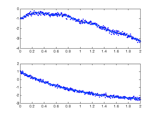
Plot Smooth with Profile-Estimated Parameters

devals = eval_fdcell(tfine,newDEfd_cell,0);
for i = 1:length(path)
    subplot(length(path),1,i)
    plot(tfine,devals{i},'r','LineWidth',2);
    hold on;
    plot(Tcell{i},Ycell{i},'b.');
    plot(plot_time,plot_path(:,i),'c');
    hold off
end

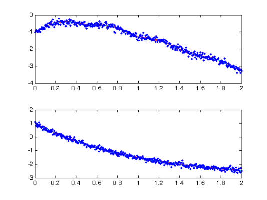
Comparison with Smooth Using True Parameters

[truecoefs,trueDEfd_cell] = genlin_smooth(path,Tcell,[],basis_cell,...
    lambda,pars,[],more);

devals = eval_fdcell(tfine,trueDEfd_cell,0);
for i = 1:length(path)
    subplot(length(path),1,i)
    plot(plot_time,plot_path(:,i),'c')
    plot(tfine,devals{i},'r','LineWidth',2);
    hold on;
    plot(plot_time,plot_path(:,i),'c');
    plot(Tcell{i},Ycell{i},'b.');
    hold off;
end

Squared Error Performance

% Squared error for estimated parameters

newpreds = eval_fdcell(Tcell,newDEfd_cell,0);
new_err = cell(length(newpreds));
for i = 1:length(path)
    new_err{i} = wts(i)*(newpreds{i} - Ycell{i}).^2;
end

new_err = mean(cell2mat(new_err));

% Squared error for true parameters


truepreds = eval_fdcell(Tcell,trueDEfd_cell,0);
true_err = cell(length(truepreds));
for i = 1:length(path)
    true_err{i} = wts(i)*(truepreds{i} - Ycell{i}).^2;
end

true_err = mean(cell2mat(true_err));

% print out a comparision

disp(['Estimated sqrd error: ',num2str(new_err)])
disp(['True sqrd error:      ',num2str(true_err)]);

Estimated sqrd error: 0.010781
True sqrd error:      0.010842

Calculate Sample Information and Variance-Covariance Matrices

% Hessian of squared error with respect to parameters

d2Jdp2 = make_d2jdp2(newDEfd_cell,fn,Ycell,Tcell,lambda,newpars,[],wts,more);

% Second derivatives with respect to parameters and observations

d2JdpdY = make_d2jdpdy(newDEfd_cell,fn,Ycell,Tcell,lambda,newpars,[],...
    wts,more);

% Resulting derivative of parameters with respect to observations

dpdY = -d2Jdp2\d2JdpdY;

% Variance of observations:

S = make_sigma(DEfd,Tcell,Ycell,0);

% Resulting parameter covariance matrix:

Cov = dpdY*S*dpdY';

%  Standard errors

StdDev = sqrt(diag(Cov));

%  Correlations

Corr = Cov./(StdDev*StdDev');

%  Display these results

disp('Approximate covariance matrix for parameters:')
disp(num2str(Cov))

disp('Approximate standard errors of parameters:')
disp(num2str(StdDev'))

disp('Approximate correlation matrix for parameters:')
disp(num2str(Corr))

Approximate covariance matrix for parameters:
  0.0055021  -0.0053143 -0.00041981  0.00027255 -0.00019605  
 -0.0053143   0.0052379   0.0004434 -0.00028756  0.00022323  
-0.00041981   0.0004434  0.00044559 -1.8669e-005  0.00020581 
 0.00027255 -0.00028756 -1.8669e-005   0.0094484 -5.0297e-006
-0.00019605  0.00022323  0.00020581 -5.0297e-006  0.00010645 
Approximate standard errors of parameters:
0.074176    0.072373    0.021109    0.097203    0.010317
Approximate correlation matrix for parameters:
       1    -0.98994    -0.26812      0.0378    -0.25617
-0.98994           1     0.29023   -0.040877     0.29896
-0.26812     0.29023           1  -0.0090986       0.945
  0.0378   -0.040877  -0.0090986           1  -0.0050154
-0.25617     0.29896       0.945  -0.0050154           1

Published with MATLAB® 7.1