Profile Estimation Experiments - the Rossler Equations
This page provides code to run profiled parameter estimation on data generated by the Rossler equations. It follows the same format as FhNEx.html and has commentary has therefore been kept to a minimum.
The Rossler equations are given by


Contents
- RHS Functions
- Various parameters
- Observation times
- Create trajectories
- Set up observations
- Fitting parameters
- Profiling optimisation control
- Setting up functional data objects
- Smooth the data
- Re-smoothing with model-based penalty
- Perform the Profiled Estimation
- Plot Smooth with Profile-Estimated Parameters
- Comparison with Smooth Using True Parameters
- Squared Error Performance
- Calculate Sample Information and Variance-Covariance Matrices
RHS Functions
odefn       = @rossfunode;    % Function for ODE solver

fn.fn       = @rossfun;       % RHS function
fn.dfdx     = @rossdfdx;      % Derivative wrt inputs
fn.dfdp     = @rossdfdp;      % Derviative wrt parameters

fn.d2fdx2   = @rossd2fdx2;    % Hessian wrt inputs
fn.d2fdxdp  = @rossd2fdxdp;   % Hessian wrt inputs and parameters
fn.d2fdp2   = @rossd2fdp2;    % Hessian wrt parameters.

fn.d3fdx3   = @rossd3fdx3;    % Third derivative wrt inputs.
fn.d3fdx2dp = @rossd3fdx2dp;  % Third derivative wrt intputs, inputs and pars.
fn.d3fdxdp2 = @rossd3fdxdp2;  % Third derivative wrt inputs, pars and pars.
Various parameters
y0 = [1.13293; -1.74953; 0.02207];       % Initial conditions

pars = [0.2; 0.2; 3];           % Parameters

sigma = 0.5;                    % Noise Level

jitter = 0.2;                                    % Perturbation for starting
startpars = pars + jitter*randn(length(pars),1); % parameter estimates
disp(['Initial par. values: ',num2str(startpars')])
Initial par. values: -0.39343 0.59033 2.6905
Observation times
tspan = 0:0.05:20;    % Observation times

obs_pts{1} = 1:length(tspan);      % Which components are observed at
obs_pts{2} = 1:length(tspan);      % which observation times.
obs_pts{3} = 1:length(tspan);


tfine = 0:0.05:20;    % Times to plot solutions
Create trajectories
odeopts = odeset('RelTol',1e-13);
[full_time,full_path] = ode45(odefn,tspan,y0,odeopts,pars);
[plot_time,plot_path] = ode45(odefn,tfine,y0,odeopts,pars);
Set up observations
Tcell = cell(1,size(full_path,2));
path = Tcell;

for i = 1:length(obs_pts)
    Tcell{i} = full_time(obs_pts{i});
    path{i} = full_path(obs_pts{i},i);
end

% add noise

Ycell = path;
for i = 1:length(path)
    Ycell{i} = path{i} + sigma*randn(size(path{i}));
end

% and set wts

wts = [];

if isempty(wts)                             % estimate wts if not given
    for i = 1:length(Ycell)
        if ~isempty(Ycell{i})
            wts(i) = 1./sqrt(var(Ycell{i}));
        else
            wts(i) = 1;
        end
    end
end
Fitting parameters
lambda  = 1e4;   % Smoothing for model-based penalty
lambda  = lambda*wts;

lambda0 = 1;     % Smoothing for 1st-derivative penalty

nknots = 401;    % Number of knots to use.
nquad  = 5;      % No. between-knots quadrature points.
norder = 3;      % Order of B-spline approximation
Profiling optimisation control
lsopts_out = optimset('DerivativeCheck','off','Jacobian','on',...
    'Display','iter','MaxIter',1000,'TolFun',1e-8,'TolX',1e-10);

% Other observed optimiation control
lsopts_other = optimset('DerivativeCheck','off','Jacobian','on',...
    'Display','iter','MaxIter',1000,'TolFun',1e-14,'TolX',1e-14,...
    'JacobMult',@SparseJMfun);

% Optimiation control within profiling
lsopts_in = optimset('DerivativeCheck','off','Jacobian','on',...
    'Display','off','MaxIter',1000,'TolFun',1e-14,'TolX',1e-14,...
    'JacobMult',@SparseJMfun);
Setting up functional data objects
% set up knots

range = [min(full_time),max(full_time)];  % range of observations

knots_cell = cell(size(path));            % knots for each basis
knots_cell(:) = {linspace(range(1),range(2),nknots)};

% set up bases

basis_cell = cell(1,length(path));    % Create cell arrays.
Lfd_cell = cell(1,length(path));

nbasis = zeros(length(path),1);

bigknots = knots_cell{1};             % bigknots used for quadrature points
nbasis(1) = length(knots_cell{1}) + norder - 2;

for i = 2:length(path)
    bigknots = [bigknots knots_cell{i}];
    nbasis(i) = length(knots_cell{i}) + norder -2;
end

quadvals = MakeQuadPoints(bigknots,nquad);   % Create simpson's rule
                                             % quadrature points and values
for i = 1:length(path)
    basis_cell{i} = MakeBasis(range,nbasis(i),norder,...  % create bases
        knots_cell{i},quadvals,1);                        % with quadrature
    Lfd_cell{i} = fdPar(basis_cell{i},1,lambda0);         % pts  attatched
end
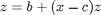
Smooth the data
DEfd = smoothfd_cell(Ycell,Tcell,Lfd_cell);
coefs = getcellcoefs(DEfd);


figure(1)
devals = eval_fdcell(tfine,DEfd,0);
for i = 1:length(path)
    subplot(length(path),1,i);
    plot(Tcell{i},Ycell{i},'b.');
    hold on;
    plot(tfine,devals{i},'r','LineWidth',2);
    if i==1
        ylabel('\fontsize{13} X')
        title(['\fontsize{13} Raw data (.), ', ...
               'and smooth fit (r-)'])
    elseif i==2
        ylabel('\fontsize{13} Y')
    else
        xlabel('\fontsize{13} t')
        ylabel('\fontsize{13} Z')
    end
end
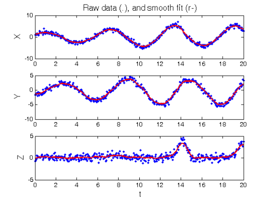
Re-smoothing with model-based penalty
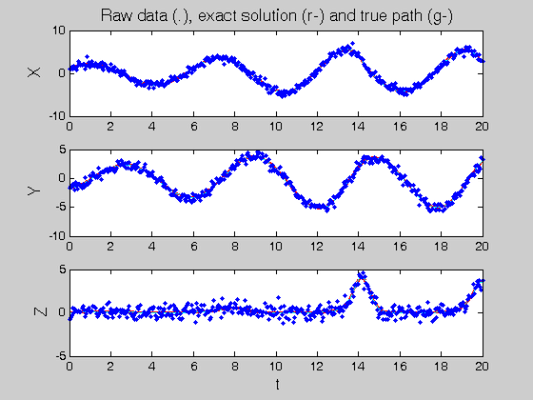
% Call the Gauss-Newton solver

[newcoefs,resnorm2] = lsqnonlin(@SplineCoefErr,coefs,[],[],lsopts_other,...
    basis_cell,Ycell,Tcell,wts,lambda,fn,[],startpars);

tDEfd = Make_fdcell(newcoefs,basis_cell);

% Plot results along with exact solution

figure(2)
devals = eval_fdcell(tfine,tDEfd,0);
for i = 1:length(path)
    subplot(length(path),1,i);
    plot(tfine,devals{i},'r','LineWidth',2);
    hold on;
    plot(Tcell{i},Ycell{i},'b.');
    plot(plot_time,plot_path(:,i),'c');
    hold off
    if i==1
        ylabel('\fontsize{13} X')
        title(['\fontsize{13} Raw data (.), ', ...
               'exact solution (r-) and true path (g-)'])
    elseif i==2
        ylabel('\fontsize{13} Y')
    else
        xlabel('\fontsize{13} t')
        ylabel('\fontsize{13} Z')
    end
end
                                         Norm of      First-order
 Iteration  Func-count     f(x)          step          optimality   CG-iterations
     0          1          394169                     2.79e+004
     1          2           99997             10      1.25e+004           20
     2          3         79828.5             20      5.63e+003          191
     3          4         46155.6             20      2.03e+004          122
     4          5         8186.78             20      7.67e+003           98
     5          6          2428.9        9.65946            457           90
     6          7         2203.72       0.618387           10.3           58
     7          8         2203.72        3.79297           10.3          298
     8          9         2199.64       0.948242           8.41            0
     9         10         2197.91        1.89648           24.3          310
    10         11         2194.57       0.120914           1.05          104
    11         12         2194.27        0.90216           15.5          307
    12         13          2194.2     0.00665249          0.363           39
    13         14         2194.19      0.0787662         0.0724          308
    14         15         2194.19     0.00788232        0.00217          308
    15         16         2194.19     0.00120445       0.000417          305
    16         17         2194.19    0.000156582      1.85e-005          310
    17         18         2194.19   2.32721e-005      3.18e-006          323
    18         19         2194.19   3.24996e-006      3.81e-007          308
Optimization terminated: relative function value
 changing by less than OPTIONS.TolFun.
Perform the Profiled Estimation
[newpars,newDEfd_cell] = Profile_GausNewt(startpars,lsopts_out,DEfd,fn,...
    lambda,Ycell,Tcell,wts,[],lsopts_in);

disp(['New parameter values: ',num2str(newpars')]);
 Iteration       steps    Residual   Improvement   Grad-norm     parameters
     1           1         1595.94      0.258366    1.45e+003     0.22024     0.10805    -0.83679
     2           1         937.855      0.412351          736     -0.11996   -0.025297    -0.60428
     3           1         574.892      0.387014          423     0.065897   -0.088672    -0.78048
     4           1         494.057       0.14061         1.23     0.077089   -0.033005    -0.68246
     5           1         364.881       0.26146         30.8     0.11369   -0.079087     0.54754
     6           1         234.323      0.357809          210     0.14755  0.00091124      2.1928
     7           1         183.119      0.218521         38.2     0.18784    0.097777      2.8046
     8           1         168.605     0.0792593         15.4     0.19623     0.19162      3.0458
     9           1         167.481     0.0066671        0.241     0.20127     0.22129      3.0709
    10           1         167.478  1.49973e-005      0.00159     0.20134     0.22207      3.0691
    11           1         167.478  2.53113e-010     0.000104     0.20134     0.22208      3.0692
New parameter values: 0.20134     0.22208      3.0692
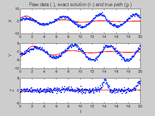
Plot Smooth with Profile-Estimated Parameters
devals = eval_fdcell(tfine,newDEfd_cell,0);
figure(3)
for i = 1:length(path)
    subplot(length(path),1,i)
    plot(tfine,devals{i},'r','LineWidth',2);
    hold on;
    plot(Tcell{i},Ycell{i},'b.');
    plot(plot_time,plot_path(:,i),'c');
    hold off
    if i==1
        ylabel('\fontsize{13} X')
        title(['\fontsize{13} Raw data (.), ', ...
               'profiled solution (r-) and true path (g-)'])
    elseif i==2
        ylabel('\fontsize{13} Y')
    else
        xlabel('\fontsize{13} t')
        ylabel('\fontsize{13} Z')
    end
end
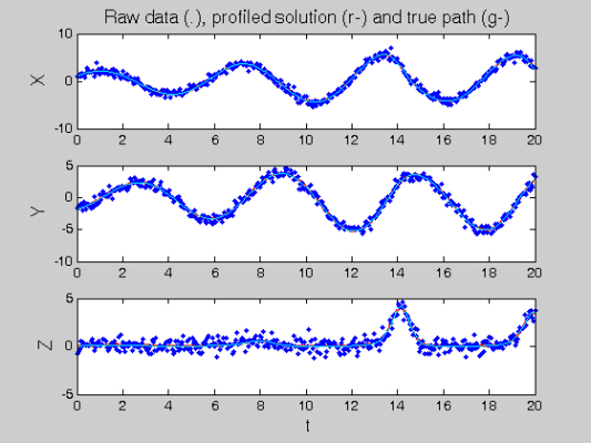
Comparison with Smooth Using True Parameters
coefs = getcellcoefs(DEfd);   % Starting coefficient estimates

[truecoefs,resnorm4] = lsqnonlin(@SplineCoefErr,coefs,[],[],...
    lsopts_other,basis_cell,Ycell,Tcell,wts,lambda,fn,[],pars);

trueDEfd_cell = Make_fdcell(truecoefs,basis_cell);

figure(4)
devals = eval_fdcell(tfine,trueDEfd_cell,0);
for i = 1:length(path)
    subplot(length(path),1,i)
    plot(plot_time,plot_path(:,i),'c')
    plot(tfine,devals{i},'r','LineWidth',2);
    hold on;
    plot(plot_time,plot_path(:,i),'c');
    plot(Tcell{i},Ycell{i},'b.');
    hold off;
    if i==1
        ylabel('\fontsize{13} X')
        title(['\fontsize{13} Raw data (.), ', ...
               'exact solution (r-) and true path (g-)'])
    elseif i==2
        ylabel('\fontsize{13} Y')
    else
        xlabel('\fontsize{13} t')
        ylabel('\fontsize{13} Z')
    end
end
                                         Norm of      First-order
 Iteration  Func-count     f(x)          step          optimality   CG-iterations
     0          1          139787                     1.52e+004
     1          2         4324.36        3.46001       1.3e+003           10
     2          3         405.558        2.58193            162           38
     3          4         196.091        2.80419            224          150
     4          5           180.1        2.50509            566          253
     5          6         170.573      0.0261129             15           13
     6          7         168.846       0.857847           8.97          365
     7          8         168.657       0.464041           16.1          493
     8          9         168.651    0.000702364          0.327           15
     9         10         168.649      0.0279744          0.101          376
    10         11         168.649     0.00890752        0.00462          548
    11         12         168.649    0.000516013       0.000127          448
    12         13         168.649    0.000129249      1.14e-005          573
    13         14         168.649    1.4119e-005       1.5e-005          603
    14         15         168.649   7.91941e-008      2.73e-006           57
Optimization terminated: relative function value
 changing by less than OPTIONS.TolFun.
Squared Error Performance
% Squared error for estimated parameters

newpreds = eval_fdcell(Tcell,newDEfd_cell,0);
new_err = cell(length(newpreds));
for i = 1:length(path)
    new_err{i} = wts(i)*(newpreds{i} - Ycell{i}).^2;
end

new_err = mean(cell2mat(new_err));

% Squared error for true parameters

truepreds = eval_fdcell(Tcell,trueDEfd_cell,0);
true_err = cell(length(truepreds));
for i = 1:length(path)
    true_err{i} = wts(i)*(truepreds{i} - Ycell{i}).^2;
end

true_err = mean(cell2mat(true_err));

% print out a comparsion

disp(['Estimated sqrd error: ',num2str(new_err)])
disp(['True sqrd error:      ',num2str(true_err)]);
Estimated sqrd error: 0.13922
True sqrd error:      0.1395
Calculate Sample Information and Variance-Covariance Matrices
% Hessian of squared error with respect to parameters

d2Jdp2 = make_d2jdp2(newDEfd_cell,fn,Ycell,Tcell,lambda,newpars,[],wts);

% Second derivatives with respect to parameters and observations

d2JdpdY = make_d2jdpdy(newDEfd_cell,fn,Ycell,Tcell,lambda,newpars,[],wts);

% Resulting derivative of parameters with respect to observations

dpdY = -d2Jdp2\d2JdpdY;

% Variance of observations:

S = make_sigma(DEfd,Tcell,Ycell,0);

% Resulting parameter covariance matrix:

Cov = dpdY*S*dpdY';

%  Standard errors

StdDev = sqrt(diag(Cov));

%  Correlations

Corr = Cov./(StdDev*StdDev');

%  Display these results

disp('Approximate covariance matrix for parameters:')
disp(num2str(Cov))

disp('Approximate standard errors of parameters:')
disp(num2str(StdDev'))

disp('Approximate correlation matrix for parameters:')
disp(num2str(Corr))
Approximate covariance matrix for parameters:
1.2131e-005 4.1516e-005    0.000128
4.1516e-005  0.00028311  0.00083986
   0.000128  0.00083986   0.0031182
Approximate standard errors of parameters:
0.003483    0.016826    0.055841
Approximate correlation matrix for parameters:
      1     0.70841     0.65813
0.70841           1     0.89386
0.65813     0.89386           1